CatiROC test GUI
Table of Contents
Intro
This project is part of the CatiROC-test group of projects. They all provide the
code necessary for testing the CatiROC ASIC from Omega.
This project comprises all the high level source code for the Matlab software. See the source code, with backups here and here.
The source code may be run from within Matlab itself, or executed as an stand alone application. This is valid under GNU/Linux as well as under windows.
This document may be used in pdf format here.
Use
Note About releases
Be aware that this software and the firmware are strongly coupled. They follow a parallel development schedule. If you decide to use a given release of this software, please use the corresponding firmware release. See the releases section of this document for more on this.
Get
Using git
This project is under source control and available as a git repository. To
download, it is necessary to have access to a git client.
- Linux users may refer to their preferred package manager for instructions on
installing
git - Windows users may use git for windows, mobaxterm of similar
Then, launch a terminal and cd to the location where the project will live,
creating necessary folders if necessary
cd d:
mkdir FolderWhereToDownload
cd FolderWhereToDownload
Finally, clone the repository with
git clone https://gitlab.in2p3.fr/CatiROC-test/gui.git catiROC-test-gui
and maybe rename it to something more explicit
mv catiROC-test-gui myGreatSoftwareProject
Direct download
Just get if from
and extract its contents; then maybe rename it to something more explicit
mv catiROC-test-gui myGreatSoftwareProject
Update
To update to the latest version (and *erase* any locally existing modifications),
use one of the git clients proposed in previous section, and then get to the
project directory
cd d:
cd FolderWhereToDownload
cd myGreatSoftwareProject
First, make a copy of all your modifications. Then, clean your working tree
with (this will *erase* all changes)
git reset --hard HEAD
and then finally pull latest project version
git pull
Start
Compatibility
The source code may be run from within MATLAB itself, or executed as an stand alone application. Executable files are provided to run under GNU/Linux as well as under windows.
The program has been tested under windows 7, centos 7 and Arch Linux. Due to the
lacky implementation of the libusb under GNU/Linux, the performances in terms of
readout bandwidth are quite poor. We have measured ~ 10 MB/s. with a recent
computer instead of ~ 40 MB/s under windows.
Matlab
The program has been developed using Matlab R2018a, but maybe new/older releases are compatible too. To run it in stand alone mode in the case R2018a is not installed locally, it is necessary first to install the correct Matlab runtime library, freely available here.
USB
In order to make the usb communication work, it is necessary to install the ftdi
libraries from here.
Run
Before running the software, remember to set the nb_asics parameter under
generic in the global configuration file accordingly to the number of asics
present in the board.
- Matlab
In a Matlab command terminal, just cd to the program and do
catirocgui
- Linux
In a GNU/Linux terminal, just cd to the program and do
./run_catirocgui.sh /opt/MATLAB/R2016a
or equivalent. You’ll probably have to deal with udev rules in your
/etc/udev/rules.d/20-ftdi.rules file or similar, as for example
SUBSYSTEM=="usb", ATTRS{idVendor}=="0403", ATTRS{idProduct}=="6010", GROUP="user", MODE="666"
Finally, you’ll maybe have to
sudo rmmod ftdi_sio; sudo rmmod usbserial
before being able to connect
- Windows
Just run the provided executable.
Project structure
Data
Using the gui, it is possible to store data on disk. In order to optimise the acquisition, reducing any data lose, data saving must disable any extra features (monitoring, histogramming, etc.) other than taking data from the hardware itself. This advised behaviour can be disabled with the SaveAndDisplay parameter.
Upon data saving, a new folder with a random name is created at the current directory, and all results are put in there. Data is saved to disk in raw format, as described below. Additionally, all configuration text files are copied to the destination folder for reference.
Regarding the binary data contents, first, a (software) header includes all necessary information to understand how the acquisition took place; then, the acquisition (hardware) data follows.
Header
The header incorporates solely information appended by the software and not originating in the hardware. It includes next fields
AcqRawDataFormatID (one byte) - Contains the acquisition (from the hardware) raw
data encoding format as provided by the firmware, see below. It is given by the
firmware in response to the command [0B, FF].
Time (seven bytes) - Acquisition start time in format
[year month day hour minute seconds]
- year
- 2 bytes
- month
- 1 byte
- day
- 1 byte
- hour
- 1 byte
- minute
- 1 byte
- seconds
- 1 byte
AsicsNb (one byte) - Number of asics in the acquisition
Command (4 times AsicNb + 2 bytes) - Contains the order user to start the
acquisition. Always starts by Ox06, followed by three times the number of asics;
ends by OxFF.
Configuration (66 times AsicNb + 2 bytes) - This includes all asics
configuration in binary format, and is equivalent to the information in the
configuration text files. Always starts by OxCC (decimal 204), followed by 66
times the number of asics; ends by OxFF.
Acquisition
Follows the acquisition (from the hardware) raw data, as explained in the
firmware page. This data is encoded following the format given by the
AcqRawDataFormatID byte, which is to be decoded as follows (in hexadecimal)
“Ox01” - version 1 of data encoding
“Ox02” - version 2 of data encoding
“Ox03” - version 3 of data encoding
Internals
Here it is included information useful to manipulate the test setup avoiding the use of the GUI, which is built up on top of what follows. This information might be useful for implementing specific tests, for developing software or for automatizing measurements with custom scripting.
First, the low level software details are provided. This remains at a C language
level, on top of which any other high level language may be used. Here, Matlab
is used as a high level framework for data manipulation and displaying.
Low level software
The low level software is coded in c. It includes functions to ease communicating with the ftdi driver, and provide an abstraction layer on top of it. Source code may be found here.
List
This is the list of valid functions provided by the low level software.
Open/close peripheral
- 'InitializeUSB'
- open the usb peripheral
- 'ConfigureUSB'
- configure the usb peripheral
- 'FinalizeUSB'
- close the usb peripheral
- 'GetIsOpen'
- check if the usb peripheral is open or not
Status
- 'GetNumberDevs'
- request number of usb peripheral on bus
- 'GetRxTxStatusUSB'
- request amount of bytes available to read
- 'GetDescriptors'
- request descriptor chain in ftdi usb eprom
Send/read
- 'ReadUSB'
- read data
- 'WriteUSB'
- send data
- 'PurgeRxTxUSB'
- send a null command and erase any trailing data in the usb low level buffers
Communication model
This section depicts the general principles about communicating with the
hardware.
The communication model is based on the following scheme. The user transfers an
array of bytes (the command) to the card using the SendCommand method. First
byte in array corresponds to the Order to be executed; remaining bytes
correspond to command parameters. Last byte is expected to always be “FF” (255
decimal).
Upon reception of a command, the card will react accordingly, stopping any
currently running action, and starting a new process. For the firmware users,
the command is written into the RegBank array within usb controller.
List of implemented commands
Note that currently commands are limited to 70 bytes, but this limit may be
removed by firmware. This software is agnostic with this respect. Follows a list
of all currently implemented functionalities in the firmware.
These commands are provided only for testing the communication with the hardware
- “01” - returns an up counter; amount of bytes is given by bytes 2 to 5 in
commandarray - “04” - returns an endless up counter
- “05” - returns the
commandsent
Next commands implement the communication with the ASIC
- “06” - returns ASIC data, used by the
“GetASICData”method - “0B” - returns the
AcqRawDataFormatIDbyte register, see Header section - “CC” - sends configuration to ASIC, used by the
“ConfigureASIC”method
Operating mode
In order to initialize the whole system of test cards, the user first needs to
create a system or TestCard object representing all test cards present in the
USB bus. Upon its creation, the software will enumerate all peripherals,
initialize and configure them. A tree of Cards objects will appear under system
structure. This way, the whole system is made available to the user
programmatically.
At this point it is then possible to address the system as a simple structure of
nested objects. Each of them will include in its properties the necessary
infrastructure to command and manipulate a given card. Data properties contain
configuration parameters, etc. Method properties include mechanism to send and
receive data, among others.
Typical session
This section includes generic instructions to initialize and finalize a working
session.
One single test board
First, load low level library in memory and give it an alias to refer to it
if ~libisloaded('libftdi')
    [notfound, warnings] = ...
        loadlibrary('libftdi_x86_4_0','libftdi_4_0.h', ...
                    'alias','libftdi')
end
Maybe, display a list of all functions available in the library
libfunctions('libftdi', '-full')
Ask for the available number of devices in the usb bus
[ft_status, NbDevices] = calllib('libftdi', 'GetNumberDevs', ...
                                 libpointer('ulongPtr',uint32(0)))
Then instantiate a TestCard object of class test_catiroc.
TestCard = test_catiroc(NbDevices-1)
which implicitly executes
TestCard.Initialize
in the class constructor.
From now on, TestCard will refer to the test card available in the usb bus, and
provides access to it, exchanging data in several different modes.
To end current session, just don’t forget to delete the TestCard object.
TestCard.delete
and unload the library from memory
if libisloaded('libftdi')
    unloadlibrary('libftdi')
end
Several test boards
Even simpler, and similar to previous case, create a system object of class
system_test.
system = system_test;
This step automatically loads the low level library in memory and instantiates a
test_catiroc class object.
From now, system will refer to all test cards available in the usb bus
(peripherals). To address one specific peripheral, refer to it by
system.Cards(1)
or simply system.Cards if there is only one card present
TestCard = system.Cards(1);
To end current session don’t forget to delete the system object
system.delete;
which removes from memory the low level library too.
Object methods
Once a TestCard object is available, the following methods allow its
manipulation.
Control methods
Check if the peripheral is open
TestCard.GetIsOpen
Check if there is any incoming data in the usb low level buffers
AmountInRxQueue = TestCard.GetStatusUSB
Obtain a string chain, describing the usb peripheral
DescChain = TestCard.GetSerialDesc
Erase any remaining trailing data
TestCard.PurgeUSB
Core i/o methods
Send command to the board
TestCard.SendCommand(Command)
Read data back
Testing methods
Proposed testing methods of the TestCard object.
Bandwidth
Measurement of data readout bandwidth, to be run NbTimes
TestCard.test_bandwidth(1, NbTimes);
Command
Test data validity. Data is assumed to contain a 8 bits up counter. This tests requests NbPackages of 65536 bytes each.
TestCard.test_command(NbPackages, 1);
Configuration methods
Update configuration data in object
TestCard = TestCard.UpdateConfig;
This parses all the configuration files and updates the object property structure with all parameters in the configuration files.
TestCard.configuration
This is useful for modifying any parameter programmatically. Thus, user may set manually any parameter
TestCard.configuration.verbose = 1;
before sending the configuration to the board
Send configuration to ASIC
TestCard.ConfigureASIC
This method will parse the
TestCard.configurationstructure, convert it to binary format and send it to the hardware.
General I/O
This section includes details on instructions to communicate (send and receive
data) with a test card.
To send (write) arbitrary data first create an array
Command = uint8([4,20,30,55,255])'; % Order X“04”
and then send it to the card
AmountBytesWritten = TestCard.SendCommand(Command);
To verify the status (amount of data available) in the USB buffers
AmountOfDataAvailable = TestCard.GetStatusUSB;
To read data available in the bus
[AmountBytesRead, BytesRead] = TestCard.ReadUSB;
To purge (delete any data present in) usb buffers
TestCards.PurgeUSB
Predefined methods for sending specific commands exist too; for example, to write random data (command X“05” = register bank) on a given length
AmountBytesWritten = TestCard.WriteRandomRB(length);
Example sessions
Configurate ASIC
This section depicts the way to configure the ASIC present in the test card.
A parameters file under configuration folder includes all configuration
registers necessary to setup the ASIC. To parse this file use
TestCard = TestCard.UpdateConfig;
This command updates the configuration object property structure. To verify the validity
of the updated configuration array use
TestCard.configuration
which is empty by default. It appears in the form of a structure, containing all fields in the parameters file. In case of more than one asic is present, do instead
TestCard.configuration(AsicNumber)
The binary representation (array of bytes) corresponding to this configuration may be found at
TestCard.configuration_array
It is used as command to be send to the board by
At this point, it is possible to send the configuration to the ASIC using
Command = TestCard.configuration_array;
and then
AmountBytesWritten = TestCard.SendCommand(Command);
See previous sections for details. Alternatively, one may just issue
AmountBytesWritten = TestCard.ConfigureASIC;
which handles sending the command to the board, reading it back and checking its validity. This may be done by hand, if considered useful using the command
There exist a reference configuration array too in the object property
TestCard.configuration_array_reference
including the default ASIC configuration at power up. This may be useful to bring the ASIC to its default status replacing previous with
Command = TestCard.configuration_array_reference;
Send ASIC slow control command
This section shows how to send slow control to the ASIC present in the test card.
Order X“CC”
system = system_test;
TestCard = system.Cards(1);
% Parse configuration file
TestCard = TestCard.UpdateConfig;
% Manually tune configuration
TestCard.configuration.parameter = value
% Should return 0
AmountInRxQueue = TestCard.GetStatusUSB
% Send configuration to hardware
BytesSent = TestCard.ConfigureASIC
system.delete;
Send random command
This section shows how to send random data to the test card.
Order X“5” will send the same data back.
system = system_test;
TestCard = system.Cards(1);
Order = 5;
% command length
L = 10;
Command = uint8([Order, 250*rand(L-2,1)', 255])
% Should return 0
AmountInRxQueue = TestCard.GetStatusUSB
% Send command, returns L
BytesSent = TestCard.SendCommand(Command)
% Should return L
AmountInRxQueue = TestCard.GetStatusUSB
% Read data back
[ElRead, DataRead] = TestCard.ReadUSB
system.delete;
Send arbitrary command
This example session shows the way to send an arbitrary, not defined command, to
the test card.
Order not implemented in firmware
system = system_test;
TestCard = system.Cards(1);
Order = 227;
% command length
L = 10;
Command = uint8([Order, 250*rand(L-2,1)', 255])
% Should return 0
AmountInRxQueue = TestCard.GetStatusUSB
% Send command, returns L
BytesSent = TestCard.SendCommand(Command)
% Should return 0
AmountInRxQueue = TestCard.GetStatusUSB
system.delete;
Read AcqRawDataFormatID
The AcqRawDataFormatID may be read from the firmware by sending the following
command to the board
Command = uint8([11, 255]);
One byte, the AcqRawDataFormatID, will be made available in return.
Take ASIC Data
In order to take data, it is necessary to use order 6 plus 4 bytes as parameters. A typical command would be the following
Command = uint8([6, ...
                 repmat([...
                     EnabledASICs, ...
                     BoardId, ...
                     ForceTriggerValue*4 + ...
                     EnableExternalTrigger*2 + ...
                     ForceTrigger, ....
                     GlobalParameters.EnableSpecialData*64 + ...
                     GlobalParameters.ReduceDiscriminatorData*32 +...
                     GlobalParameters.EnablePhysicalData*16 +...
                     GlobalParameters.EnableDiscriminatorData*8 +...
                     GlobalParameters.DecodeGray*4 + ...
                     str2double(obj.configuration(1).EnableTacReadout)*2 + ...
                     emulate], ...
                        1, nb_asics), ...
                 255])';
where
Byte one:
- EnabledASICs
- one byte, one bit by asic, providing an enable / disable functionality for masking data from given asics
Byte two:
- BoardId
- one byte to identify this board; all data will be tagged with this byte which will appear in last byte in every event
Byte three:
- Bit[13-10] ForceTriggerValue
- selects the force trigger rate (default to 0), see Fake trigger section for more on this
- Bit[9] EnableExternalTrigger
- activates the external trigger (default to 1)
- Bit[8] ForceTrigger
- activate the forcetrigger feature in the firmware (default to 0)
Byte four:
- Bit[6] EnableSpecialData
- activates special data readout
- Bit[5] ReduceDiscriminatorData
- activates DDS data reduction (default to 0)
- Bit[4] EnablePhysicalData
- activates the physical data stream (default to 1)
- Bit[3] EnableDiscriminatorData
- activates the discriminator data stream (default to 1)
- Bit[2] DecodeGray
- activates the gray decoding feature in firmware, as data out of the ASIC is gray encoded (default to 1)
- Bit[1] EnableTacReadout
- parameter from the configuration file (default to 1)
- Bit[0] Emulate
- activates the “bypass of catiroc” feature in the firmware (default to 0)
Note that here, between the order 6 and the trailing FF the (4 bytes)
parameters are replicated number of asics times. This is important to be
compliant with the firmware.
TODO Take S-Curve Data
In order to take s-curve data, it is necessary to …
Command = uint8([6, ...
                 repmat([...
                     emulate], ...
                        1, obj.nb_asics), ...
                 255])';
Where …
Configuration
General information
The configuration files follow the following rules
Config parameters are given as
- VARIABLE = VALUE; # COMMENT
Comment lines take the format
All text after # is considered as a comment
Empty lines are allowed
- … and ignored
Catiroc parameters files
There exists one configuration file by asic. They are numbered from 1 to
nb_asics.
catiroc_parameters_1.param
catiroc_parameters_2.param
…
The “format” suffix in "VARIABLE-format" stands for the format representation of VARIABLE. Valid options are ’bin’, ’hex’ and ’dec’
Example:
Variable = 10 (dec)
Variable = 1010 (bin, most significant bit to the left)
Variable = A (hex, most significant bit to the left)
Take into account that in binary fields, most significant bit goes to the left so that “1000”/hex“8” (and not bin“0001”/hex“1” !!) is equivalent to decimal 8.
In the case of Omega documentation, a 16 bits register A from bit 0 to bit 15 is assigned as follows:
Bit 0 contient le bit de poids fort
Bit 15 contient le bit de poids faible
… but not always. When decoding the configuration file, attention has been payed so as to deal with this feature carefully.
Global configuration file
Generic
Juno mezzanine board has eight asics, whereas omega test board has only one.
nb_asics = 8;
For debugging purposes during development
verbose = 0;
Acq
Id tag to be appended to all évents as its last byte
BoardId = 1;
It is possible to display some acquisition related informations while acquiring data (event and data rate, decoded fields of the first events by data package, etc.).
This parameter sets the number of events to display in command window at run time
ToDisplay = 0;
where
- 0
- no events to display
- <5
- only special events
- >5
- this number of events
There exists the possibility to save data on disk and compute/display histograms at the same time. This feature is enabled by using this parameter. It is disabled by default as data lose is expected to occur in this case (cpu resources are taken and not available for acquiring and saving data)
SaveAndDisplay = 0;
This parameter forces mixing up data from two analog memories (ping and pong) in displayed histograms
Randomize = 0;
This parameter sets the number of bytes in a data package to ask for to the usb. It must be an integer multiple of 10. See No data !! section for its effects.
AmountInRxQueue = 65540;
Allow decoding online the default format out of the asic, gray encoding, in the firmware, converting it on the fly to unsigned binary.
DecodeGray = 1;
Enable discriminator data or not. When disabled, discriminator data is just discarded in the firmware
EnableDiscriminatorData = 1;
Reduce discriminator data. When enabled, discriminator data is compressed to a single word, instead of the default of two words by event
ReduceDiscriminatorData = 0;
Enable physical data or not. When disabled, physical data is just discarded in the firmware
EnablePhysicalData = 1;
Enable special data or not. When disabled, special data is just discarded in the firmware
EnableSpecialData = 1;
Enabled ASIC, in hexadecimal format, one bit by ASIC, going from ASIC[8] to the left down to ASIC[1], to the right.
EnabledASICs = "FF";
Force trigger rate: maximum rate is 15. Refer to Fake trigger section for details
ForceTrigRate = 15;
Enable exteral trigger
EnableExternalTrigger = 1;
Ignore fake events from the ASIC; set to zero not to ignore. See Fake events section for details.
IgnoreFakeEvents = 1;
Osc
Not implemented in firmware. To ignore.
PacketSize = 2^16;
S-Curve
See S-Curve computing for details.
Minimum, maximum and step values for the threshold
s_curve.th.min = 940;
s_curve.th.step = 2;
s_curve.th.max = 1020;
Methods used:
- Method = 1 -> Use data
- Method = 0 -> Use trigger
s_curve.method = 0;
Number of of periods to average
s_curve.nb_periods = 100;
INL
TimingINL.steps = 300;
TimingINL.time = 10;
Analysis
When performing data analysis, there is the possibility to only analyse a fix number of events. This parameter sets the number of (10 bytes) events to analyse at the beginning of the data file.
Set it to -1 to analyse the whole file
NbEventsToAnalyse = -1;
Tips
Collection of unrelated issues specific to a given functionalities.
Fake events
D’un autre coté, je constate que CatiROC envoie un événement nul systématiquement à chaque démarrage: j’arrive pas à corriger cet effet. Manque d’idées, on va considérer pour le moment ceci comme un fait. En attendant, il faudra le corriger par soft (ou pas). Pour cela, il faut savoir que chaque moitié de CatiROC (1-8 ou bien 9-16) enverra un événement nul. Pour les éliminer il faudra, d’abord, compter combien il y en a (suivant la configuration choisie, numéro d’asics actifs et masques sur les voies). Ensuite, il faudra passer à les éliminer en sachant qu’ils font partie des événements physiques, et qu’ils sont à zéro. J’ai implémenté la correction à mode d’exemple/vérification sur mon soft d’acquisition / analyse.
Fake trigger
It is possible to force CatiROC to take data regardless of the analog input signals. This is possible by using the available fake trigger feature: CatiROC takes de logical OR of the channel local discriminator output (local trigger) with an external signal, the “fake” trigger.
Two variants of this feature are implemented:
- force trigger
- using the gui, select the chekbox to send a fpga-generated periodic pulse to CatiROC acting as its fake trigger. This signal will send by default a 30 KHz periodic pulse to the asic. It is possible to reduce this frequency by tunning the number (0 by default) in the gui close to the “force trigger” check box up to a maximum of 15 (meaning 1 KHz). 1
- external trigger
- a positive polarity signal plugged into the
io_fpga1SMA input of the test board will be routed to CatiROC fake trigger input
Even if probably useless, it is possible to use both possibilities.
Buffering resources and dead time
Following discussion concerns exclusively Juno mezzanine board. It is related to eventual data lose observed during the acquisition.
First, recall that
- measured USB2 readout bandwidth is
~40 MB/s.under windows - buffering ressources are estimated to be
1152 KB(biggest block is 128 KB times 9 Bytes)
Then, considering data rate, a force trigger signal of X KHz will produce
Xe3 (KHz) * 3 (data sources) * 10 (Bytes/trigger) * 128 (channels)
bytes per second. As a motivating example, at 1 KHz we get
1e3 * 3 * 10 * 128 / (1024*1024)
3.662109375
MB/s.
Now, considering a data rate of N MB/s. the buffering within the Kindex 7 FPGA
may store up to
1152 / (N*1024)
seconds worth of data before saturating buffers. Following the previous example, this gives
1152 / (3.66*1024)
0.3073770491803279
seconds of buffering resources. This means that data taking may stop during this time without any (acquisition) dead time. These stop time slots may arise from control cpu usage, usb low level internals, etc.
Finally, note that these figures are coherent with results presented here.
USB communication
Fine Time characterization
Release 0.8 implements the possibility to perform a systematic scan of the (25 ns.) coarse time window. This provides a way to measure the fine time INL as shown in the next figure.
Context
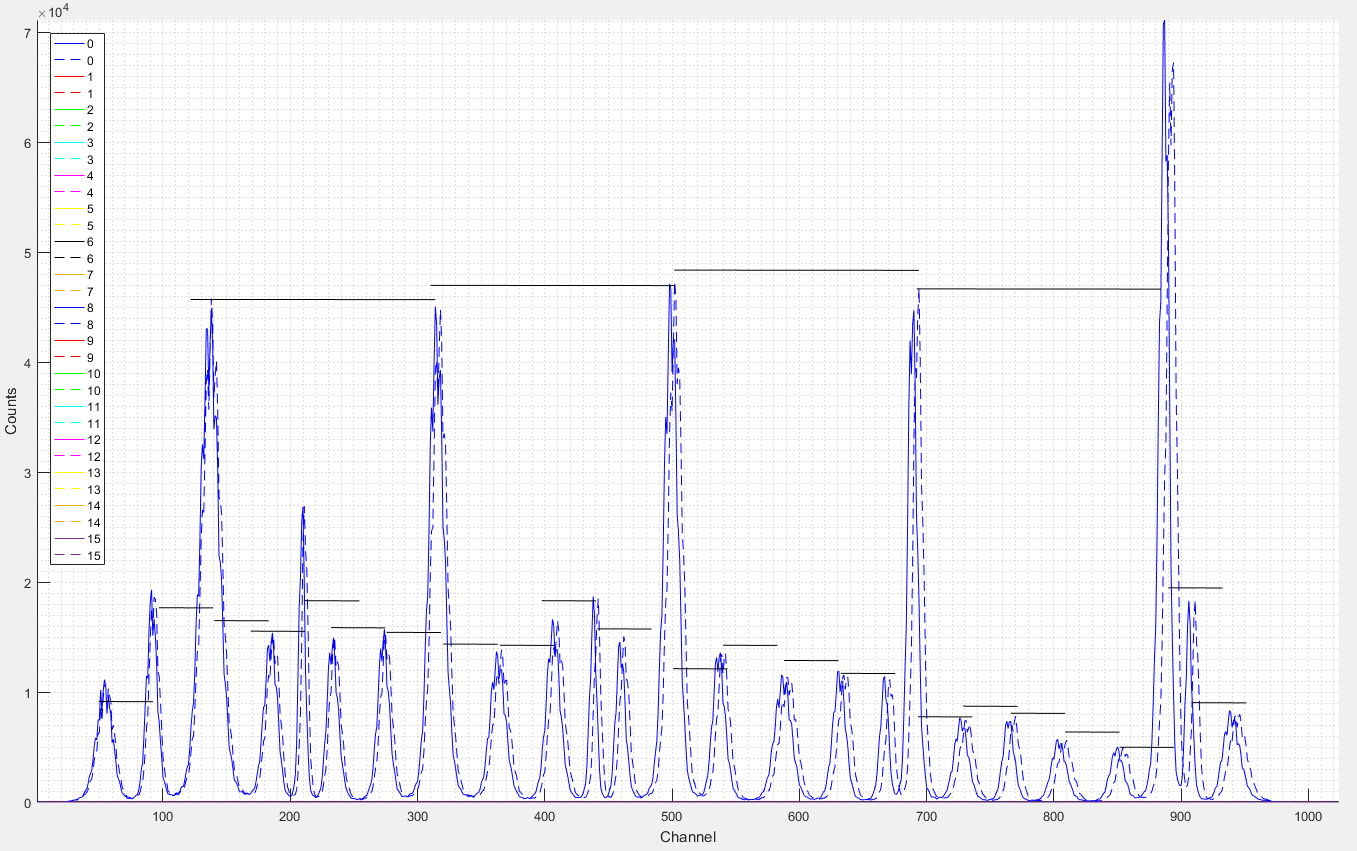
This plot is obtained by injecting a constant amplitude signal from a pulse generator, and going through an attenuator to improve SNR. The generator is in sync with the 10 MHz clock of the acquisition, providing a constant measurement of the fine time. This means that we are able to inject a signal from the pulse generator and obtain always the same fine time. Histogramming this measurement provides the resulting gaussian shape, corresponding to a fix time delay setup in the pulse generator.
At this point, adding a delay makes the gaussian shape shift accordingly. Thus, by manually increasing the pulse generator delay in 1 ns. steps we manage to shift the measurement to the left, producing 25 (one by ns.) shifted versions of the same measurement.
Note that a 30 ns. delay is equivalent to a 5 ns. delay due to the periodic 25 ns. coarse time window length.
Horizontal black lines are shown here as a rough reference: they are all the same length (long ones equal 5 ns., and short ones 1 ns.). This provides a first impression of how linear the fine time is when increasing the delay by 1 ns. steps.
Extension
Release 0.8 firmware embeds a variable, configurable 97.65 ps digital delay line to replace the manual delay in the pulse generator. This is possible as the delay line acts on the 10 MHz to be sent from the acquisition to the external pulse generator. This replaces the need to manually tune the generator delay parameter.
This effectively provides a means to perform a custom, systematic software scan by programmatically setting the delay steps of the measurement. Fine time characterization has thus been included in release 0.8 software. Details are given below.
Setup
In order to reproduce previous plot, and to further execute a scan of
the coarse time window, the following steps are to be followed (note
that tests were done using a AFG-3022B pulse generator form Tektronix)
set the following parameter in the configuration file
SelClkDiv4 = 0;This forces the ASIC to use the 40 MHz clock from the fpga, effectively removing any ambiguity otherwise. This means that when catiROC generates a 40 MHz clock using the 160 MHz from the fpga, there exists four different possibilities to lock the former with respect to the later. This random behaviour will repeat at each ASIC reset, that’s to say, at each data taking. Sending the 40 MHz clock to catiROC erases this random behaviour, which is an issue in this context
- connect output
io_fpga10to an oscilloscope, and outputio_fpga9to the trigger input of the pulse generator - setup the pulse generator using an internal reference (continuous
mode) to output a pulse of the desired frequency and amplitude;
start taking data as usual to check data is coming, note how in
io_fpga10at the oscilloscope a 10 MHz clock signal appears after the acquisition starts: you’ll get the same fromio_fpga9, and you’ll notice how the green led lights on - lock the pulse generator to its 10 MHz clock trigger input (burst mode), and check at the oscilloscope how the 10 MHz clock and the generated pulse are synchronous now
- plug the pulse from the generator to the board and visualize the fine time histogram, where a gaussian shape corresponding to a fixed fine time value should be appreciated
- set the pulse generator delay parameter; the digital delay line will add a delay starting from this point
From here, scanning the coarse time window is a matter of selecting in
the Tools menu the Time INL option. Here, the number of 97.65
ps. steps to be used for the scanning is given by the TimingINLsteps
parameter in the global parameters configuration file, while the scan
time is given in the TimingINLtime in the same file. For example,
setting this to 30 and 10 (default values), will perform a 10 seconds
data acquisition, before increasing the delay by 97.65 ps steps and
then taking data again. One binary data file will be stored on disk by
delay.
TODO:
Software for analysis the data.
TODO:
Ancillary soft to the gui.
S-Curve computing
The S-Curve computing feature is included starting from version 1.9. It allows obtaining the s-curves of all channels in parallel. Results are displayed, and may be also saved on disk for further analysis.
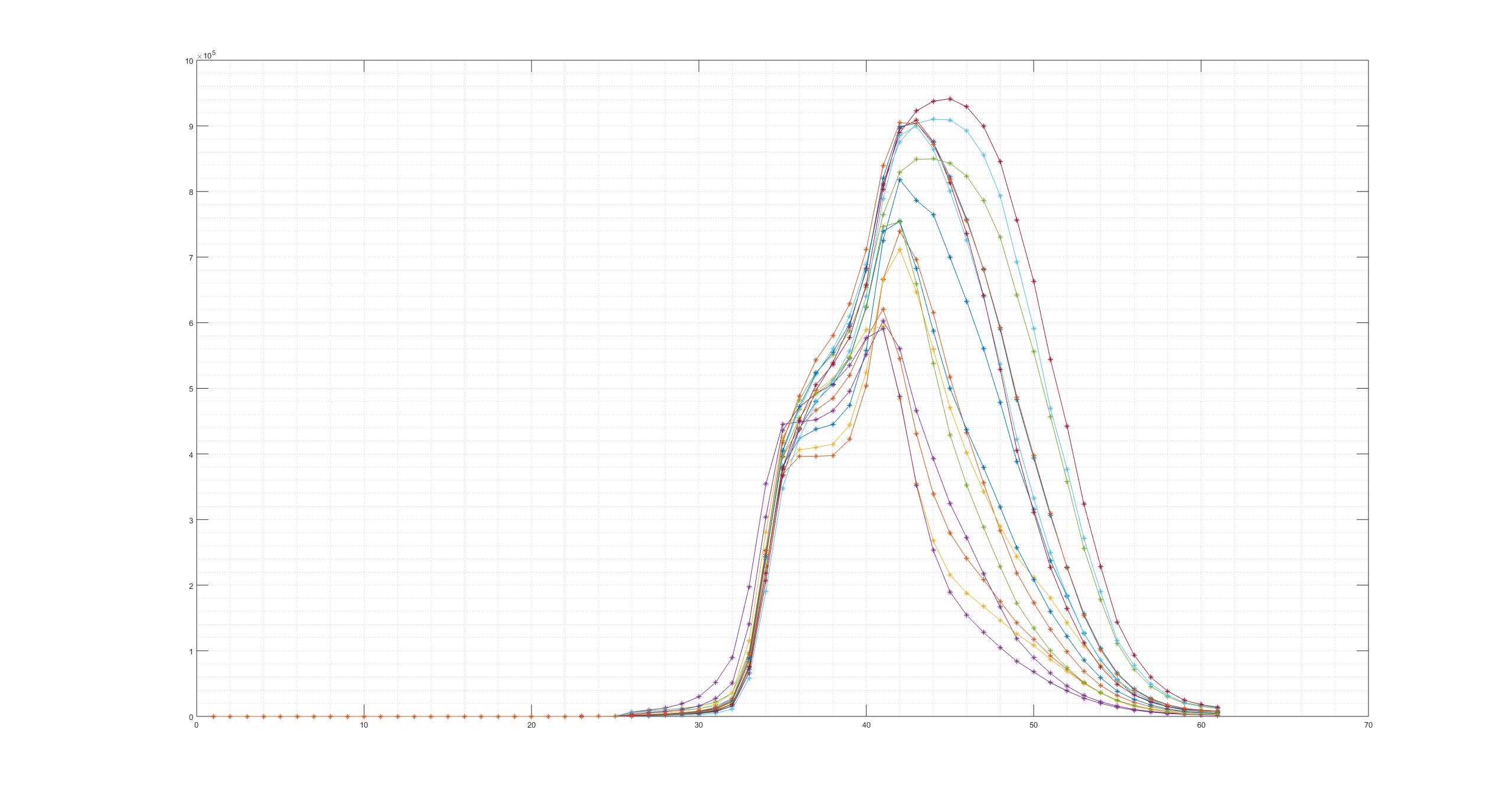
Figure 2: One ASIC, 16 channels S-Curves computed using triggers
This feature is composed of a firmware implementation, along with manipulation by software of the computed data in order to correctly present it.
Within the firmware, the embedded algorith will perform a sampling of a signal over a ~12.5 ms. period every 12.5 ns. This signal, by channel, may be
- the trigger output of the ASIC
- new incoming data signal generated in the firmware when a new event is detected
This way, the algorithm counts the number of occurrencies of this signal within
an arbitraty length 12.5 ms time window (2^20 counts @ 80 MHz), sampling signal
levels every 12.5 ns., which makes 2^20 samples. The number of total counts
measured is readout to the software, which averages over a number of 12.5 ms
periods (nb_periods).
Before launching the s-curve, the acquisition parameters must be setup in the case the readout data is to be used. This is achieved by launching previously a dummy acquisition as usual, with the desired parameters (no force trigger, enabled physical data, etc.)
Withing the software, it is possible to perform an automated scan, computing the
s-curve, starting from a minimum threshold (s_curve.th.min) up to a maximum
(s_curve.th.max), using a given step (s_curve.th.step).
The s_curve.method to be used is sampling the trigger (0) signal or the data
signal (1), being the trigger the outputs of the ASIC discriminator, while data
are the readout events detected in the firmware. Note that the former is
(almost) dead time free, while the later strongly depends on the data rate and
the number of active channels. Finally, it is possible to average the
measurement, making the results less sensible to noise, by repeating it over
s_curve.nb_periods consecutive 12.5 ms time windows.
All these parameters are to be setup in the global_parameters.param file.
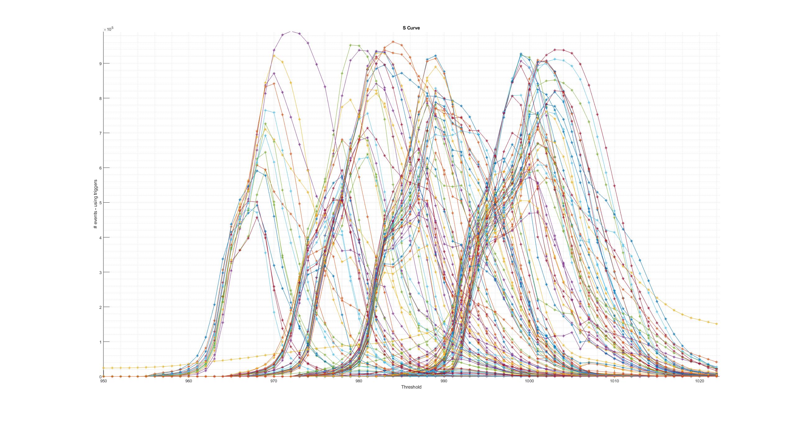
Figure 3: Eight ASICs, 128 channels S-Curves computed using triggers
Releases
Be aware that this software and the firmware are strongly coupled. They follow a parallel development schedule. If you decide to use a given release of this software, please use the corresponding firmware release.
As a reference, releases may be found here
- software
- https://gitlab.in2p3.fr/CatiROC-test/gui/tags
- firmware
- https://gitlab.in2p3.fr/CatiROC-test/firmware/tags
Releases provide new features or bug fixes.
X
TODO Include here all previous modifications
0.7
0.8
0.9
1.0
1.1
Disable DDS by software
- Bit to disable the feature
- DDR makes amount of data to be readout rise beyond limits, specially considering the usb 2. Add a bit to command 6 to disable this feature when requested by the user.
- OK
- Done in this commit, in parallel to the software.
1.2
1.3
1.4
1.5
1.6
1.7
1.8
TODO-List
List of next to do items: ideas, new features, corrections, improvements, etc.
TODO Multi board mode
- … bla
TODO Cli mode
Checking List
List of to be checked items: new implemented features, etc.
TODO S-curve, save data
- Current implementation
- check that the current implementation is right, for both omega test board and ABC board
- Store data on disk
- Use the ’Save Data’ button to store on disk the resulting data from the s-curve scanning. Create a new dir, picking-up its name from a parameter in the global config file (if this parameter is empty, just create a random folder name), and put data in here similar to the standard acquisition. Save .mat and .txt files, along with the figures in .fig and .tiff and .jpeg formats. Implement in the figure manual saving of the curves using the right mouse button
Bugs and features
A list of current bugs to be fixed and requested features may be found under the open issues list in the online project.
Troubleshooting
No data !!
Under some conditions, a message claiming that no incoming data exist may appear. This is due to the way data is acquired: the software ask for a given amount of data, in bytes, as for the parameter in the “global_configuration” file
AmountInRxQueue = 2^16;
When this number of bytes is not sent from the board before a few seconds, the “no data !!” message is displayed. Then, the acquisition waits for a few more seconds. If not enough data arrives, it just stops.
The reason for this to happen may be a high threshold, a low count rate or any other reason decreasing the data rate. To fix the issue in case of low data rate, you may modify this parameter by decreasing its value, but it must remain a multiple of 10 (so 65000, 60000 are accepted values)
AmountInRxQueue = 65540;
Note that this will have an effect in terms of data transfer rate, as big data packages are necessary to maximize the overall rate, so for high counting (data) rates, better use the default.
Finally, you may check the maximum data rate using the Tools menu.
Fine time data shifts
Note that the value of the parameter
SelClkDiv4
will make shift the fine time values. This may be observed using the fine time histogram when acquiring data asynchronously.
License
This program is free software; you can redistribute it and/or modify it under the terms of the GNU General Public License as published by the Free Software Foundation, either version 3 of the License, or (at your option) any later version.
This program is distributed in the hope that it will be useful, but WITHOUT ANY WARRANTY; without even the implied warranty of MERCHANTABILITY or FITNESS FOR A PARTICULAR PURPOSE. See the GNU General Public License for more details.
You should have received a copy of the GNU General Public License along with this program. If not, see http://www.gnu.org/licenses/gpl.html.
Footnotes:
To compute the frequency from this field use the formula
(60e6)/(hex2dec("N800")*1e3)
where “N” stands for the field close to the “force trigger” check box.